HYGOV

HYGOV is a hydro turbine-governor model with temporary droop, a gate servo, and a nonlinear single-penstock turbine.

Warning

HYGOVD dbL/dbH, mechanical backlash (db2), and Kaplan blade-servo behavior are not modeled. Nonzero db2 values log a warning and are ignored.

Notes

None.

Block Diagram

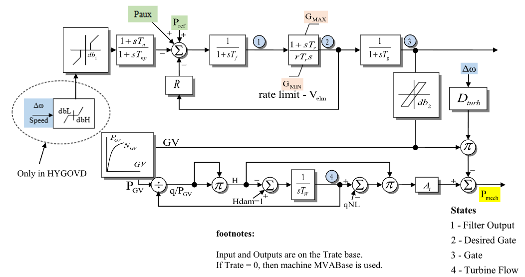
Figure 1: HYGOV governor model. Figure courtesy of the PowerWorld HYGOV model reference.

Model Parameters

Symbol	Units	JSON	Description	Typical Value	Note
\(T^\mathrm{rate}\)	[MW]	Trate	Turbine-rating power base	100.0	Required
\(R_{\mathrm{perm}}\)	[p.u.]	Rperm	Permanent droop	0.04	Source label: R
\(R_{\mathrm{temp}}\)	[p.u.]	Rtemp	Temporary droop	0.3	Source label: r
\(T_\mathrm{r}\)	[s]	Tr	Temporary-droop reset time constant	5.0
\(T_\mathrm{f}\)	[s]	Tf	Governor error filter time constant	0.05
\(T_\mathrm{g}\)	[s]	Tg	Gate servo time constant	0.5
\(V_{\mathrm{elm}}\)	[p.u./s]	Velm	Maximum desired-gate velocity magnitude	0.2
\(G^{\max}\)	[p.u.]	Gmax	Configured upper gate response limit	1.0
\(G^{\min}\)	[p.u.]	Gmin	Configured lower gate response limit	0.0
\(T_\mathrm{w}\)	[s]	Tw	Water inertia time constant	1.0
\(A_\mathrm{t}\)	[p.u.]	At	Turbine gain	1.2
\(D_{\mathrm{turb}}\)	[p.u.]	Dturb	Turbine damping coefficient	0.5
\(q_{\mathrm{NL}}\)	[p.u.]	Qnl	No-load flow at nominal head	0.05
\(T_\mathrm{n}\)	[s]	Tn	Speed lead–lag numerator time constant	0.0
\(T_{\mathrm{np}}\)	[s]	Tnp	Speed lead–lag denominator time constant	0.0
\(D_{\omega}\)	[p.u.]	db1	Type 1 speed deadband threshold	0.0
\(D_2\)	[p.u.]	db2	Unsupported mechanical backlash deadband	0.0	Nonzero values warn and are ignored
\(H_{\mathrm{dam}}\)	[p.u.]	Hdam	Configured dam head	1.0	Lower bound on effective head
\(G_V^{(k)}\)	[p.u.]	Gv0-Gv5	Gate point \(k\) of the gain curve	0.0	\(k=0,\ldots,5\)
\(P_{\mathrm{GV}}^{(k)}\)	[p.u.]	Pgv0-Pgv5	Power point \(k\) of the gain curve	0.0	\(k=0,\ldots,5\)

Real-valued parameters accept real or integer JSON values. All-zero Gv and Pgv source points select the identity curve.

Parameter Validation

A valid HYGOV parameter set must satisfy the following conditions:

\[\begin{split}\begin{aligned} T^\mathrm{rate} &> 0 \\ T_\mathrm{r}, T_\mathrm{f}, T_\mathrm{g}, T_\mathrm{w}, T_{\mathrm{np}} &\ge 0 \\ R_{\mathrm{temp}} &> 0 \\ T_\mathrm{n} &\ge 0 \\ V_{\mathrm{elm}} &\ge 0 \\ G^{\min} &< G^{\max} \\ A_\mathrm{t} &> 0 \\ D_{\mathrm{turb}} &\ge 0 \\ D_{\omega} &\ge 0 \\ H_{\mathrm{dam}} &> 0 \\ G_V^{(k)} &< G_V^{(k+1)} \quad k\in\{0,\ldots,4\} \\ P_{\mathrm{GV}}^{(k)} &\le P_{\mathrm{GV}}^{(k+1)} \quad k\in\{0,\ldots,4\} \\ G_V^{(0)} \le G^{\min} &< G^{\max} \le G_V^{(5)} \\ P_\mathrm{m}(G_V^{(5)}) - P_\mathrm{m}(G_V^{(0)}) &> \epsilon_{\mathrm{init}} \end{aligned}\end{split}\]

Real-valued parameters, Known initial values, power bases, and base-conversion ratios must be finite. The bases and ratios must also be positive.

The final condition uses the steady mechanical power and tolerance defined under Internal Initialization.

Model Derived Parameters

Let \(\epsilon_T=10^{-3}\ \mathrm{s}\). A time constant below \(\epsilon_T\) is raised to that floor in place, so every equation below uses the raised value:

\[\begin{split}\begin{aligned} T_x &\leftarrow \max\!(T_x,\epsilon_T), \quad x\in\{r,f,g,w,\mathrm{np}\} \\ k_{\mathrm{base}} &= \dfrac{S^\mathrm{sys}}{10^6\,T^\mathrm{rate}} \\ k_\mathrm{n} &= \dfrac{T_\mathrm{n}}{T_{\mathrm{np}}} \\ N_{\mathrm{GV}}(x) &= P_{\mathrm{GV}}^{(0)} + \sum_{k\in\{0,\ldots,4\}} \text{linseg}\!( x;\, G_V^{(k)},\, G_V^{(k+1)},\, P_{\mathrm{GV}}^{(k+1)} - P_{\mathrm{GV}}^{(k)} ) \end{aligned}\end{split}\]

Multiplying by \(k_\mathrm{base}\) converts system base to component base; \(S^\mathrm{sys}\) is the system power base in VA.

Model Ports

Name	Port	Init	Description
speed	Input	Known	Machine speed deviation
pref	Input	Unknown	Active-power/load reference
paux	Input	Known	Auxiliary power input
pmech	Output	Known	Mechanical power output

Known values are seeded before initialization and preserved. Unknown inputs are initialized in attached signal storage or held constant when unattached. The pmech output must be assigned. The signal inputs are optional. Unattached speed and paux inputs default to zero.

Model Variables

Internal Variables

Differential

Symbol	Units	Description	Note
\(x_\mathrm{n}\)	[p.u.]	Speed lead–lag denominator state	Not circled in Fig. 1. Realizes the Tn/Tnp block
\(x_\mathrm{f}\)	[p.u.]	Governor error filter output	State 1 in Fig. 1
\(c\)	[p.u.]	Desired-gate position	State 2 in Fig. 1
\(g\)	[p.u.]	Gate position	State 3 in Fig. 1
\(q\)	[p.u.]	Turbine flow	State 4 in Fig. 1

Algebraic

Symbol	Units	Description	Note
\(\omega_{\mathrm{db}}\)	[p.u.]	Type 1 deadbanded speed deviation
\(e_f\)	[p.u.]	Governor error into the filter	Reference path less conditioned speed and permanent-droop feedback
\(f_c\)	[p.u./s]	Desired-gate derivative target	Before rate and position limits
\(r_c\)	[p.u./s]	Rate-limited desired-gate derivative target	Limited by \(\pm V_{\mathrm{elm}}\)
\(P_{\mathrm{GV}}\)	[p.u.]	Nonlinear gate-to-power curve output	\(N_{\mathrm{GV}}(g)\)
\(H\)	[p.u.]	Turbine head	Implicit water-column head
\(P_\mathrm{m}\)	[p.u.]	Mechanical power to generator	System base

External Variables

Differential

None.

Algebraic

Symbol	Units	Description	Note
\(\omega\)	[p.u.]	Machine speed deviation	Optional signal port speed. Defaults to zero
\(P^\mathrm{ref}\)	[p.u.]	Active-power/load reference	Optional signal port pref, system base
\(P^\mathrm{aux}\)	[p.u.]	Auxiliary power input	Optional signal port paux, system base, defaults to zero

Model Equations

Smooth functions: antiwindup, clamp, deadband1, linseg.

Internal Equations

Differential

The effective desired-gate response limits \(G_{\mathrm{resp}}^{\min}\) and \(G_{\mathrm{resp}}^{\max}\) and the effective dam head \(H_{\mathrm{dam}}^{\mathrm{eff}}\) are resolved during initialization.

\[\begin{split}\begin{aligned} 0 &= -\dot{x}_n + \dfrac{1}{T_{\mathrm{np}}} (\omega_{\mathrm{db}} - x_\mathrm{n}) \\ 0 &= -\dot{x}_f + \dfrac{1}{T_\mathrm{f}} (e_f - x_\mathrm{f}) \\ 0 &= -\dot{c} + \text{antiwindup} (c, r_c;\, G_{\mathrm{resp}}^{\min}, G_{\mathrm{resp}}^{\max}) \\ 0 &= -\dot{g} + \dfrac{1}{T_\mathrm{g}} (c - g) \\ 0 &= -\dot{q} + \dfrac{1}{T_\mathrm{w}} (H_{\mathrm{dam}}^{\mathrm{eff}} - H) \end{aligned}\end{split}\]

Algebraic

\[\begin{split}\begin{aligned} 0 &= -\omega_{\mathrm{db}} + \text{deadband1} (\omega;\, -D_{\omega}, D_{\omega}) \\ 0 &= -e_f + k_{\mathrm{base}}(P^\mathrm{ref} + P^\mathrm{aux}) - x_\mathrm{n} - k_\mathrm{n}(\omega_{\mathrm{db}} - x_\mathrm{n}) - R_{\mathrm{perm}}c \\ 0 &= -R_{\mathrm{temp}}f_c + \dfrac{x_\mathrm{f}}{T_\mathrm{r}} + \dfrac{e_f - x_\mathrm{f}}{T_\mathrm{f}} \\ 0 &= -r_c + \text{clamp} (f_c;\, -V_{\mathrm{elm}}, V_{\mathrm{elm}}) \\ 0 &= -P_{\mathrm{GV}} + N_{\mathrm{GV}}(g) \\ 0 &= -q^2 + H P_{\mathrm{GV}}^2 \\ 0 &= -k_{\mathrm{base}}P_\mathrm{m} + A_\mathrm{t} H(q - q_{\mathrm{NL}}) - D_{\mathrm{turb}}\omega g \end{aligned}\end{split}\]

External Equations

None.

Initialization

Input Initialization

\[\begin{split}\begin{aligned} \omega &\leftarrow \text{machine speed deviation} \\ P_\mathrm{m} &\leftarrow \text{machine mechanical power on system base} \\ P^\mathrm{aux} &\leftarrow \text{auxiliary power input on system base} \end{aligned}\end{split}\]

Initialization never replaces the system-base value held in \(P_\mathrm{m}\).

Internal Initialization

Initialization requires an exactly zero speed deviation, \(\omega = 0\). Restart initialization of a moving machine is not supported. All internal derivatives are set to zero.

Initialization first solves the gate at the configured dam head over the full \([G_V^{(0)},G_V^{(5)}]\) gate curve. If that gate lies outside the configured \([G^{\min},G^{\max}]\) interval, the corresponding response limit is expanded to include it. The configured parameters are unchanged. This matches PowerWorld’s default Modify Limits and Run treatment of initial limit violations.

If the required mechanical power exceeds the value at \(G_V^{(5)}\), the gate is pinned there and an effective dam head \(H_{\mathrm{dam}}^{\mathrm{eff}} \ge H_{\mathrm{dam}}\) is raised to reproduce the operating point. Both searches use the same smooth \(N_{\mathrm{GV}}\) curve as the residual. No upper limit is applied to the head adjustment. The effective values remain the response limits and water-column setpoint during simulation.

\[\begin{split}\begin{aligned} H &\leftarrow H_{\mathrm{dam}}^{\mathrm{eff}} \\ g &\leftarrow \text{gate in } [G_V^{(0)},G_V^{(5)}] \text{ satisfying} \\ &\qquad k_{\mathrm{base}}P_\mathrm{m} = A_\mathrm{t} H\left(\sqrt{H}\,N_{\mathrm{GV}}(g) - q_{\mathrm{NL}}\right) \\ G_{\mathrm{resp}}^{\min} &\leftarrow \min\!(G^{\min},g) \\ G_{\mathrm{resp}}^{\max} &\leftarrow \max\!(G^{\max},g) \\ P_{\mathrm{GV}} &\leftarrow N_{\mathrm{GV}}(g) \\ q &\leftarrow \sqrt{H}\,P_{\mathrm{GV}} \\ c &\leftarrow g \\ \omega_{\mathrm{db}} &\leftarrow \text{deadband1}\!(\omega;\, -D_{\omega}, D_{\omega}) \\ x_\mathrm{n} &\leftarrow \omega_{\mathrm{db}} \\ x_\mathrm{f} &\leftarrow 0 \\ e_f &\leftarrow 0 \\ f_c &\leftarrow 0 \\ r_c &\leftarrow 0 \end{aligned}\end{split}\]

A value within \(\epsilon_{\mathrm{init}} = 100\,\epsilon_{\mathrm{mach}}\) below the \(G_V^{(0)}\) endpoint initializes at \(G_V^{(0)}\) with a mechanical-power residual up to \(\epsilon_{\mathrm{init}}\). A lower value, or a high-side value without a finite effective dam head, is rejected. All other accepted values initialize with every residual at machine rounding.

Every check resolves before state, the effective response limits, the effective dam head, or signals are written, so a rejected initialization leaves them unchanged.

Output Initialization

\[\begin{aligned} P^\mathrm{ref} &\leftarrow \dfrac{1}{k_{\mathrm{base}}} \left[ e_f - k_{\mathrm{base}}P^\mathrm{aux} + x_\mathrm{n} + k_\mathrm{n}(\omega_{\mathrm{db}} - x_\mathrm{n}) + R_{\mathrm{perm}}c \right] \end{aligned}\]

Monitors

Monitor	Units	Description	Note
pmech	[p.u.]	Mechanical-power output	\(P_\mathrm{m}\) (system base)
filter	[p.u.]	Governor error filter output	\(x_\mathrm{f}\) (component base)
desiredgate	[p.u.]	Desired-gate position	\(c\) (component base)
gate	[p.u.]	Gate position	\(g\) (component base)
flow	[p.u.]	Turbine flow	\(q\) (component base)
head	[p.u.]	Turbine head	\(H\) (component base)

Appendix A: Backlash

Input \(u\), output \(y\), half-play \(b\), with \(|u - y| \le b\).

\[\begin{split}\begin{aligned} \dot{y} &= \begin{cases} \dot{u} & |u - y| = b \text{ and } \dot{u}(u - y) > 0 \\ 0 & \text{otherwise} \end{cases} \end{aligned}\end{split}\]

which can be written in terms of our smooth functions as

\[\begin{aligned} 0 &= -\dot{y} + \text{ramp}(\dot{u})\,\text{above}(u - y;\, b) - \text{ramp}(-\dot{u})\,\text{below}(u - y;\, -b) \end{aligned}\]

CommonMath defines the ramp, above, and below targets and smooth approximations. This is deferred until we permit non Hessenberg forms. Once permitted we should define:

\[\begin{aligned} \text{backlash}(u,\dot{u},y;b) &= \text{ramp}(\dot{u})\,\text{above}(u - y;\, b) - \text{ramp}(-\dot{u})\,\text{below}(u - y;\, -b) \end{aligned}\]