REGCA

REGCA is a first-generation WECC renewable generator/converter model for inverter-coupled resources.

Notes

None.

Block Diagram

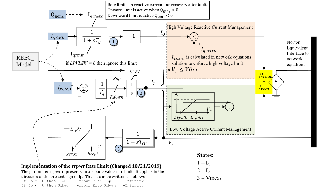
Figure 1: REGCA generator/converter model. Figure courtesy of the PowerWorld REGC_A model reference.

Model Parameters

Symbol	Units	JSON	Description	Typical Value	Note
\(P_0\)	[p.u.]	p0	Initial active power injection	1.0	System base; required initialization source
\(Q_0\)	[p.u.]	q0	Initial reactive power injection	0.0	System base; required initialization source
\(S^\mathrm{base}\)	[MVA]	mva	REGCA component power base	100.0
\(T_\mathrm{g}\)	[s]	Tg	Converter current-control lag time constant	0.02
\(T_M\)	[s]	TM	Terminal voltage sensor time constant	0.02	Source label: Tfltr
\(R_q^{\max}\)	[p.u./s]	Rqmax	Reactive-current recovery positive rate limit	999.0	Source label: Iqrmax; disabled when \(R_q^{\max}\le 0\)
\(R_q^{\min}\)	[p.u./s]	Rqmin	Reactive-current recovery negative rate limit	-999.0	Source label: Iqrmin; disabled when \(R_q^{\min}\ge 0\)
\(R_p^{\max}\)	[p.u./s]	Rpmax	Active-current magnitude recovery rate limit	999.0	Source label: rrpwr; must be nonnegative
\(s_L\)	[binary]	sL	LVPL switch	1	Source label: LPVLSW
\(I_{L1}\)	[p.u.]	IL1	LVPL upper-current ceiling	1.1	Source label: LVPL1
\(V_{L0}\)	[p.u.]	VL0	LVPL zero-crossing voltage	0.4	Source label: zerox
\(V_{L1}\)	[p.u.]	VL1	LVPL upper breakpoint voltage	0.9	Source label: brkpt
\(V_{A0}\)	[p.u.]	VA0	LVACM lower breakpoint voltage	0.4	Source label: LVPnt0
\(V_{A1}\)	[p.u.]	VA1	LVACM upper breakpoint voltage	0.9	Source label: LVPnt1
\(V_\mathrm{hv}^{\max}\)	[p.u.]	Vhvmax	HV reactive management activation threshold	1.2	Source label: VLim
\(Q^{\min}\)	[p.u.]	Qmin	PowerWorld compatibility field		Optional; accepted but unused
\(K_\mathrm{hv}\)	[p.u.]	Khv	HV reactive management gain	0.7	Optional; defaults to 0.7; block name: Khv
\(X_\mathrm{e}\)	[p.u.]	Xe	PowerWorld compatibility field		Optional; accepted but unused

All listed JSON parameters are required unless marked optional.

Parameter Validation

A valid REGCA parameter set must satisfy the following conditions:

\[\begin{split}\begin{aligned} \epsilon_T &= 10^{-3} \\ T &\leftarrow \max(T, \epsilon_T) \quad T\in\{T_\mathrm{g},T_M\} \\ S^\mathrm{base} &> 0 \\ R_p^{\max} &\ge 0 \\ I_{L1} &\ge 0 \\ K_L &> 0 \\ s_L &\in \{0,1\} \\ 0 &\le V_{L0} < V_{L1} \\ 0 &\le V_{A0} < V_{A1} < V_\mathrm{hv}^{\max} \\ 0 \le K_\mathrm{hv} &< \infty \end{aligned}\end{split}\]

Time constants below \(\epsilon_T\) are raised to \(\epsilon_T\) and logged as a warning, every other condition is a configuration error.

Model Derived Parameters

\[\begin{split}\begin{aligned} s_L^\mathrm{off} &= 1 - s_L \\ k_\mathrm{base} &= \dfrac{S^\mathrm{sys}}{S^\mathrm{base}} \\ K_L &= 100 \end{aligned}\end{split}\]

The fixed slope \(K_L\) [p.u./p.u.] approximates the unbounded LVPL characteristic above \(V_{L1}\).

Model Ports

Name	Port	Init	Description
bus	Bus	Known	Terminal bus voltage
ipcmd	Input	Unknown	Active-current command input
iqcmd	Input	Unknown	Reactive-current command input
ibranchr	Output	Known	Branch-current real-component output
ibranchi	Output	Known	Branch-current imaginary-component output
pbranch	Output	Known	Branch active-power output
qbranch	Output	Known	Branch reactive-power output

Model Variables

Internal Variables

Differential

Symbol	Units	Description	Note
\(V_M\)	[p.u.]	Filtered terminal voltage	State 3 in Fig. 1
\(I_q\)	[p.u.]	Reactive-current state	State 1 in Fig. 1 before the -1 block; component base
\(I_p\)	[p.u.]	Active-current state	State 2 in Fig. 1; component base

Algebraic

Symbol	Units	Description	Note
\(V_T\)	[p.u.]	Terminal voltage magnitude
\(I_r\)	[p.u.]	Branch-current real component	System base
\(I_i\)	[p.u.]	Branch-current imaginary component	System base
\(I_q^\mathrm{extra}\)	[p.u.]	Extra inductive current from high-voltage reactive current management	Component base
\(I_L\)	[p.u.]	LVPL upper-limit current curve	Component base; function of \(V_M\)
\(P^\mathrm{br}\)	[p.u.]	Branch active power	System base
\(Q^\mathrm{br}\)	[p.u.]	Branch reactive power	System base

External Variables

Differential

None.

Algebraic

Symbol	Units	Description	Note
\(V_r\)	[p.u.]	Terminal voltage, real component	Bus input
\(V_i\)	[p.u.]	Terminal voltage, imaginary component	Bus input
\(I_p^\mathrm{cmd}\)	[p.u.]	Active-current command in the terminal-voltage reference frame	Optional signal port ipcmd; system base
\(I_q^\mathrm{cmd}\)	[p.u.]	Reactive-current command in the terminal-voltage reference frame	Optional signal port iqcmd; system base

Model Equations

Smooth functions: clamp, linseg, max, min, \(\rho\).

Define the pre-limit current derivatives:

\[\begin{split}\begin{aligned} f_\mathrm{q} &= \dfrac{1}{T_\mathrm{g}} (k_\mathrm{base} I_q^\mathrm{cmd} - I_q) \\ f_\mathrm{p} &= \dfrac{1}{T_\mathrm{g}} (k_\mathrm{base} I_p^\mathrm{cmd} - I_p) \end{aligned}\end{split}\]

Figure 1 places LVPL on the active-current integrator ceiling, realized by the awmax gate in the differential equations. The ceiling moves with the sensed voltage, and a pinned \(I_p\) tracks it as a non-windup limit. rrpwr applies the active-current recovery rule according to the sign of \(I_p\).

The limited active-current integrator drive applies the recovery rate rule of Appendix A:

\[f_\mathrm{p}^{\lim} = \text{rrpwr}(I_p, f_\mathrm{p}; R_p^{\max})\]

Internal Equations

Differential

The \(I_q\) limiter branch is selected by the configured reactive power \(Q_0\) and the sign that enables the corresponding limit.

\[\begin{split}\begin{aligned} 0 &= -\dot V_M + \dfrac{1}{T_M} (V_T - V_M) \\ 0 &= -\dot I_q + \begin{cases} \text{min}(f_\mathrm{q}, R_q^{\max}) & Q_0 > 0 \land R_q^{\max} > 0 \\ \text{max}(f_\mathrm{q}, R_q^{\min}) & Q_0 < 0 \land R_q^{\min} < 0 \\ f_\mathrm{q} & \text{otherwise} \end{cases} \\ 0 &= -\dot I_p + \begin{cases} f_\mathrm{p}^{\lim} & s_L = 0 \\ \text{awmax}(I_p, f_\mathrm{p}^{\lim}; I_L, \dot I_L) & s_L = 1 \end{cases} \end{aligned}\end{split}\]

Algebraic

\[\begin{split}\begin{aligned} 0 &= -V_T^2 + V_r^2 + V_i^2 \\ 0 &= -k_\mathrm{base} V_T I_r + V_i(I_q - I_q^\mathrm{extra}) + V_r I_p\,\text{linseg}(V_T; V_{A0}, V_{A1}, 1) \\ 0 &= -k_\mathrm{base} V_T I_i - V_r(I_q - I_q^\mathrm{extra}) + V_i I_p\,\text{linseg}(V_T; V_{A0}, V_{A1}, 1) \\ 0 &= -I_q^\mathrm{extra} + K_\mathrm{hv}\,\text{ramp}(V_T - V_\mathrm{hv}^{\max}) \\ 0 &= -I_L + \text{linseg}(V_M; V_{L0}, V_{L1}, I_{L1}) + K_L\,\text{ramp}(V_M - V_{L1}) \\ 0 &= -P^\mathrm{br} + V_r I_r + V_i I_i \\ 0 &= -Q^\mathrm{br} + V_i I_r - V_r I_i \end{aligned}\end{split}\]

External Equations

\[\begin{split}\begin{aligned} I_r^\mathrm{inj} &:= I_r \\ I_i^\mathrm{inj} &:= I_i \end{aligned}\end{split}\]

Initialization

Input Initialization

\[\begin{split}\begin{aligned} V_r,V_i &\leftarrow \text{terminal-bus voltage} \\ P_0,Q_0 &\leftarrow \text{power-flow injection on system base} \end{aligned}\end{split}\]

Internal Initialization

Initialization requires \(V_{A1}\le V_T\) and, with LVPL enabled, \(I_p\le I_L\). All internal derivatives initialize to zero.

\[\begin{split}\begin{aligned} V_T &\leftarrow \sqrt{V_r^2+V_i^2} \\ V_M &\leftarrow V_T \\ I_L &\leftarrow \text{linseg}(V_T;V_{L0},V_{L1},I_{L1}) +K_L\,\text{ramp}(V_T-V_{L1}) \\ I_p &\leftarrow \dfrac{k_\mathrm{base}P_0}{V_T\,\text{linseg}(V_T;V_{A0},V_{A1},1)} \\ I_q^\mathrm{extra} &\leftarrow K_\mathrm{hv}\,\text{ramp}(V_T-V_\mathrm{hv}^{\max}) \\ I_q &\leftarrow \dfrac{k_\mathrm{base}Q_0}{V_T}+I_q^\mathrm{extra} \\ I_r &\leftarrow \dfrac{V_rP_0+V_iQ_0}{V_T^2} \\ I_i &\leftarrow \dfrac{V_iP_0-V_rQ_0}{V_T^2} \\ P^\mathrm{br} &\leftarrow P_0 \\ Q^\mathrm{br} &\leftarrow Q_0 \end{aligned}\end{split}\]

Output Initialization

\[\begin{split}\begin{aligned} I_p^\mathrm{cmd} &\leftarrow \dfrac{I_p}{k_\mathrm{base}} \\ I_q^\mathrm{cmd} &\leftarrow \dfrac{I_q}{k_\mathrm{base}} \end{aligned}\end{split}\]

Monitors

Monitor	Units	Description	Note
ir	[p.u.]	Real current injection	System base; exported through ibranchr when assigned
ii	[p.u.]	Imaginary current injection	System base; exported through ibranchi when assigned
p	[p.u.]	Active-power output	System base; exported through pbranch when assigned
q	[p.u.]	Reactive-power output	System base; exported through qbranch when assigned

Appendix A: rrpwr

The exact active-current rate-limit rule is

\[\begin{split}\text{rrpwr}(x, f; r) = \begin{cases} \text{max}(f, -r) & x < 0 \\ \text{clamp}(f; -r, r) & x = 0 \\ \text{min}(f, r) & x > 0 \end{cases}\end{split}\]

The model evaluates this rule with the following continuously differentiable (\(C^1\)) approximation:

\[\begin{split}\begin{aligned} t(x) &= \tanh\!\left(\dfrac{\mu x}{2}\right)=2\sigma(x)-1 \\[0pt] w_+(x) &= \dfrac{t(x)^2+t(x)\lvert t(x)\rvert}{2} \\[0pt] w_-(x) &= \dfrac{t(x)^2-t(x)\lvert t(x)\rvert}{2} \\[0pt] \text{rrpwr}(x,f;r) &\approx f +\left[1-w_+(x)\right]\text{ramp}(-f-r) -\left[1-w_-(x)\right]\text{ramp}(f-r) \end{aligned}\end{split}\]

Where \(\sigma\) is GridKit’s smooth sigmoid. The one-sided weights and their first derivatives vanish at \(x=0\). The approximation therefore equals slew exactly at zero and preserves the outward rate limit for finite \(\mu\) while gradually releasing restoring motion.

Appendix B: awmax

The exact anti-windup rule under a moving upper bound \(u\) with rate \(\dot u\) is

\[\begin{split}\text{awmax}(x, f; u, \dot u) = \begin{cases} f & x < u \\ \text{min}(f, \dot u) & x \ge u \end{cases}\end{split}\]

Below the bound the unconstrained derivative passes. Pinned at the bound, the state tracks \(\text{min}(f, \dot u)\), so a falling bound drags the state down with it. The rule is fixed-bound anti-windup on the gap \(g = x - u\) held below zero: pinned, \(\dot g = \text{min}(f - \dot u, 0) \le 0\), so the gap cannot grow and closes whenever \(f < \dot u\).

The model evaluates this rule with the following smooth approximation:

\[\text{awmax}(x, f; u, \dot u) \approx \dot u + \left[\sigma(u-x)+(1-\sigma(u-x))\sigma(\dot u-f)\right] (f - \dot u)\]

With a stationary bound (\(\dot u = 0\)) this reduces to the antiwindup of CommonMath restricted to its upper limit, which admits an algebraic bound \(u\).