EXPIC1

EXPIC1 is a proportional/integral excitation system with terminal-voltage sensing, a PI regulator, cascaded regulator filters, stabilizing feedback, potential/current-source scaling, rectifier loading, exciter limits, saturation, and an exciter field-voltage state.

Warning

The PI proportional path, regulator output limits, \(T_E=0\) bypass, and initialization still need reconciliation with the source diagram.

Notes

• Internal voltage and current signals are on model base unless otherwise stated.

• The rectifier loading block \(F_{\mathrm{ex}}=f(I_N)\) is the source AC-exciter loading curve from Fig. 1; it is not a CommonMath helper.

• If \(K_P=0\) and \(K_I=0\), the diagram sets \(V_B=1\).

• If \(T_E=0\), the source diagram states \(E_{\mathrm{fd}}=E_0\); the exciter field state becomes algebraic.

Block Diagram

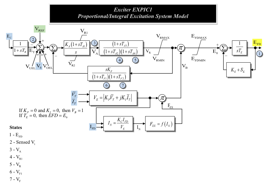
Figure 1: Exciter EXPIC1 model. Figure courtesy of PowerWorld

Model Parameters

Symbol	Units	JSON	Description	Typical Value	Note
\(T_R\)	[s]	Tr	Transducer time constant	0.0	if zero, \(E_T\) is algebraic
\(K_A\)	[p.u.]	Ka	PI regulator gain	1.0
\(T_{A1}\)	[s]	Ta1	PI regulator numerator time constant	0.0
\(V_{R1}^{\max}\)	[p.u.]	Vr1	PI regulator upper output limit	1.0	Source label: VR1
\(V_{R2}^{\min}\)	[p.u.]	Vr2	PI regulator lower output limit	-1.0	Source label: VR2
\(T_{A2}\)	[s]	Ta2	First denominator time constant in regulator filter	0.0
\(T_{A3}\)	[s]	Ta3	Numerator time constant in regulator filter	0.0
\(T_{A4}\)	[s]	Ta4	Second denominator time constant in regulator filter	0.0
\(V_R^{\max}\)	[p.u.]	Vrmax	Maximum regulator output before source multiplier	1.0
\(V_R^{\min}\)	[p.u.]	Vrmin	Minimum regulator output before source multiplier	-1.0
\(K_F\)	[p.u.]	Kf	Stabilizing feedback gain	0.0
\(T_{F1}\)	[s]	Tf1	First feedback denominator time constant	0.0
\(T_{F2}\)	[s]	Tf2	Second feedback denominator time constant	0.0
\(E_{\mathrm{fd}}^{\max}\)	[p.u.]	Efdmax	Maximum exciter input limit	5.0	Source label: EFDMAX
\(E_{\mathrm{fd}}^{\min}\)	[p.u.]	Efdmin	Minimum exciter input limit	-5.0	Source label: EFDMIN
\(K_E\)	[p.u.]	Ke	Exciter field-resistance line-slope margin	0.1
\(T_E\)	[s]	Te	Exciter time constant	0.5	if zero, \(E_{\mathrm{fd}}=E_0\)
\(E_1\)	[p.u.]	E1	First saturation voltage point	2.8
\(S_E(E_1)\)	[p.u.]	SE1	Saturation value at \(E_1\)	0.08	Source label: Se1
\(E_2\)	[p.u.]	E2	Second saturation voltage point	3.7
\(S_E(E_2)\)	[p.u.]	SE2	Saturation value at \(E_2\)	0.33	Source label: Se2
\(K_P\)	[p.u.]	Kp	Potential-source voltage coefficient	0.0	Source label: KP; forms \(V_E\)
\(K_I\)	[p.u.]	Ki	Potential-source current coefficient	0.0	Source label: KI; forms \(V_E\)
\(K_C\)	[p.u.]	Kc	Rectifier loading current coefficient	0.0	forms \(I_N\)

Parameter Validation

A valid EXPIC1 parameter set must satisfy the following conditions:

\[\begin{split}\begin{aligned} &T_R \ge 0,\quad T_{A1}\ge 0,\quad T_{A2}\ge 0,\quad T_{A3}\ge 0,\quad T_{A4}\ge 0 \\ &T_{F1}\ge 0,\quad T_{F2}\ge 0,\quad T_E\ge 0 \\ &V_{R2}^{\min}\le V_{R1}^{\max},\quad V_R^{\min}\le V_R^{\max},\quad E_{\mathrm{fd}}^{\min}\le E_{\mathrm{fd}}^{\max} \end{aligned}\end{split}\]

The saturation points are either disabled together or define a valid positive two-point quadratic fit.

Model Derived Parameters

The saturation curve is fitted from the two supplied saturation points. If both saturation factors are zero, use \(S_A=0\) and \(S_B=0\). Otherwise:

\[\begin{split}\begin{aligned} C &= \sqrt{\dfrac{S_E(E_2)}{S_E(E_1)}} \\ S_A &= \dfrac{C E_1 - E_2}{C - 1} \\ S_B &= \dfrac{S_E(E_1)}{(E_1 - S_A)^2} \end{aligned}\end{split}\]

The source voltage components are:

\[\begin{split}\begin{aligned} V_{\mathrm{src}}^r &= K_P V_r - K_I I_i \\ V_{\mathrm{src}}^i &= K_P V_i + K_I I_r \end{aligned}\end{split}\]

Model Ports

Name	Port	Init	Description
ec	Input	TBD	Compensated terminal voltage magnitude \(E_C\)
vref	Input	TBD	Voltage-control reference \(V_{\mathrm{ref}}\)
vuel	Input	TBD	Under-excitation limiter input \(V_{\mathrm{uel}}\)
vs	Input	TBD	Stabilizer input signal \(V_S\)
voel	Input	TBD	Over-excitation limiter input \(V_{\mathrm{oel}}\)
vr	Input	TBD	Terminal-voltage real component \(V_r\)
vi	Input	TBD	Terminal-voltage imaginary component \(V_i\)
ir	Input	TBD	Terminal-current real component \(I_r\)
ii	Input	TBD	Terminal-current imaginary component \(I_i\)
ifd	Input	TBD	Machine field current \(I_{\mathrm{fd}}\)
efd	Output	TBD	Field-voltage output \(E_{\mathrm{fd}}\)

Model Variables

Internal Variables

Differential

Symbol	Units	Description	Note
\(E_{\mathrm{fd}}\)	[p.u.]	Field-voltage output state	State 1 in Fig. 1; algebraic when \(T_E=0\)
\(E_T\)	[p.u.]	Sensed terminal voltage	State 2 in Fig. 1; Source label: Sensed Vt; algebraic when \(T_R=0\)
\(V_A\)	[p.u.]	PI regulator output	State 3 in Fig. 1
\(x_{R1}\)	[p.u.]	First regulator filter state	State 4 in Fig. 1; Source label: VR1
\(V_R\)	[p.u.]	Regulator output before source multiplier	State 5 in Fig. 1; Source label: VR
\(V_{F1}\)	[p.u.]	First feedback filter state	State 6 in Fig. 1; Source label: VF1
\(V_F\)	[p.u.]	Stabilizing feedback output	State 7 in Fig. 1; Source label: VF

Algebraic

Symbol	Units	Description	Note
\(e_V\)	[p.u.]	Voltage-error signal after feedback	Summing junction after \(E_T\)
\(V_{\mathrm{src}}^r\)	[p.u.]	Real component of the source expression	From terminal voltage/current components
\(V_{\mathrm{src}}^i\)	[p.u.]	Imaginary component of the source expression	From terminal voltage/current components
\(V_{\mathrm{src}}\)	[p.u.]	Potential/current source magnitude	Nonnegative source magnitude
\(I_N\)	[p.u.]	Normalized exciter loading current	Source label: IN; satisfies \(V_{\mathrm{src}}I_N=K_C I_{\mathrm{fd}}\) when source scaling is active
\(F_{\mathrm{ex}}\)	[p.u.]	Rectifier loading factor	Source label: FEX; source curve \(F_{\mathrm{ex}}=f(I_N)\)
\(V_B\)	[p.u.]	Source multiplier after rectifier loading	Product of \(V_{\mathrm{src}}\) and \(F_{\mathrm{ex}}\), or 1 when \(K_P=K_I=0\)
\(E_0\)	[p.u.]	Limited exciter input	Limited by \(E_{\mathrm{fd}}^{\min}\) and \(E_{\mathrm{fd}}^{\max}\)
\(S_E\)	[p.u.]	Saturation coefficient evaluated at \(E_{\mathrm{fd}}\)	Uses derived saturation curve

External Variables

Differential

None.

Algebraic

Symbol	Units	Description	Note
\(E_C\)	[p.u.]	Compensated terminal voltage magnitude	Source label: EC
\(V_{\mathrm{ref}}\)	[p.u.]	Voltage-control reference	Source label: VREF
\(V_{\mathrm{uel}}\)	[p.u.]	Under-excitation limiter input	Source label: VUEL; optional, defaults to zero
\(V_S\)	[p.u.]	Stabilizer input signal	Source label: VS; optional, defaults to zero
\(V_{\mathrm{oel}}\)	[p.u.]	Over-excitation limiter input	Source label: VOEL; optional, defaults to zero
\(V_r\)	[p.u.]	Terminal-voltage real component	Source label: VT
\(V_i\)	[p.u.]	Terminal-voltage imaginary component	Source label: VT
\(I_r\)	[p.u.]	Terminal-current real component	Source label: IT
\(I_i\)	[p.u.]	Terminal-current imaginary component	Source label: IT
\(I_{\mathrm{fd}}\)	[p.u.]	Machine field current	Source label: IFD

Model Equations

Smooth functions: antiwindup, clamp, \(q\).

Internal Equations

Differential

\[\begin{split}\begin{aligned} 0 &= -T_R\dot E_T - E_T + E_C \\ 0 &= -\dot V_A + \text{antiwindup}\!( V_A, K_A e_V; V_{R2}^{\min}, V_{R1}^{\max} ) \\ 0 &= -T_{A2}\dot x_{R1} - x_{R1} + V_A \\ 0 &= -T_{A4}\dot V_R - V_R + x_{R1} + T_{A3}\dot x_{R1} \\ 0 &= -T_{F1}\dot V_{F1} - V_{F1} + V_R \\ 0 &= -T_{F2}\dot V_F - V_F + K_F\dot V_{F1} \\ 0 &= -T_E\dot E_{\mathrm{fd}} + E_0 - (K_E + S_E)E_{\mathrm{fd}} \end{aligned}\end{split}\]

Algebraic

\[\begin{split}\begin{aligned} 0 &= -e_V + V_{\mathrm{ref}} + V_{\mathrm{uel}} + V_S + V_{\mathrm{oel}} - E_T - V_F \\ 0 &= -V_{\mathrm{src}}^r + K_P V_r - K_I I_i \\ 0 &= -V_{\mathrm{src}}^i + K_P V_i + K_I I_r \\ 0 &= -V_{\mathrm{src}}^2 + (V_{\mathrm{src}}^r)^2 + (V_{\mathrm{src}}^i)^2 \\ 0 &= \begin{cases} -I_N & K_P=0\ \text{and}\ K_I=0 \\ -V_{\mathrm{src}}I_N + K_C I_{\mathrm{fd}} & \text{otherwise} \end{cases} \\ 0 &= -F_{\mathrm{ex}} + \begin{cases} 1 & K_P=0\ \text{and}\ K_I=0 \\ f(I_N) & \text{otherwise} \end{cases} \\ 0 &= -V_B + \begin{cases} 1 & K_P=0\ \text{and}\ K_I=0 \\ V_{\mathrm{src}}F_{\mathrm{ex}} & \text{otherwise} \end{cases} \\ 0 &= -E_0 + \text{clamp}(V_B V_R; E_{\mathrm{fd}}^{\min}, E_{\mathrm{fd}}^{\max}) \\ 0 &= -S_E + S_B\,q(E_{\mathrm{fd}} - S_A) \end{aligned}\end{split}\]

The \(V_{\mathrm{src}}\) residual uses the nonnegative branch of the squared source-magnitude equation.

External Equations

None.

Initialization

For a standard unsaturated start, the machine initializes \(E_{\mathrm{fd}}\) and \(I_{\mathrm{fd}}\) first. EXPIC1 reads those values, sets all internal derivatives to zero, and evaluates:

\[\begin{split}\begin{aligned} E_T &\leftarrow E_C \\ V_{\mathrm{src}}^r &\leftarrow K_P V_r - K_I I_i \\ V_{\mathrm{src}}^i &\leftarrow K_P V_i + K_I I_r \\ V_{\mathrm{src}} &\leftarrow \sqrt{ (V_{\mathrm{src}}^r)^2 + (V_{\mathrm{src}}^i)^2 } \\ I_N &\leftarrow \begin{cases} 0 & K_P=0\ \text{and}\ K_I=0 \\ \dfrac{K_C I_{\mathrm{fd}}}{V_{\mathrm{src}}} & \text{otherwise} \end{cases} \\ F_{\mathrm{ex}} &\leftarrow \begin{cases} 1 & K_P=0\ \text{and}\ K_I=0 \\ f(I_N) & \text{otherwise} \end{cases} \\ V_B &\leftarrow \begin{cases} 1 & K_P=0\ \text{and}\ K_I=0 \\ V_{\mathrm{src}}F_{\mathrm{ex}} & \text{otherwise} \end{cases} \\ S_E &\leftarrow S_B\,q(E_{\mathrm{fd}} - S_A) \\ E_0 &\leftarrow (K_E + S_E)E_{\mathrm{fd}} \\ V_R &\leftarrow \dfrac{E_0}{V_B} \\ x_{R1} &\leftarrow V_R \\ V_A &\leftarrow x_{R1} \\ V_{F1} &\leftarrow V_R \\ V_F &\leftarrow 0 \\ e_V &\leftarrow \dfrac{V_A}{K_A} \\ V_{\mathrm{ref}} &\leftarrow e_V + E_T + V_F - V_{\mathrm{uel}} - V_S - V_{\mathrm{oel}} \end{aligned}\end{split}\]

This closed-form start requires nonzero \(K_A\) and \(V_B\), inactive PI and exciter limits, and residual consistency with the source curve. When \(K_P\) and \(K_I\) are not both zero, it also requires \(V_{\mathrm{src}}\ne 0\). If \(T_E=0\), the final exciter residual is algebraic and requires \(E_{\mathrm{fd}}=E_0\). Starts that bind the PI regulator, cascaded regulator, or exciter limits are outside these closed-form equations.

Monitors

Monitor	Units	Description	Note
efd	[p.u.]	Field-voltage output	\(E_{\mathrm{fd}}\)
et	[p.u.]	Sensed terminal voltage	\(E_T\)
va	[p.u.]	PI regulator state	\(V_A\)
vr1	[p.u.]	First regulator filter state	\(x_{R1}\)
vr	[p.u.]	Regulator output	\(V_R\)
vf1	[p.u.]	First feedback filter state	\(V_{F1}\)
vf	[p.u.]	Stabilizing feedback output	\(V_F\)
vb	[p.u.]	Source multiplier	\(V_B\)
in	[p.u.]	Normalized exciter loading current	\(I_N\)
fex	[p.u.]	Rectifier loading factor	\(F_{\mathrm{ex}}\)
se	[p.u.]	Saturation coefficient	\(S_E\)