StateSpace

StateSpace represents a vector-fitted matrix rational approximation with real or complex poles and factorized residue terms. For pole count \(Q\), define the pole-index set

\[\mathcal{Q} = \{q \in \mathbb{Z}_{>0} \mid q \le Q\}\]

\[\mathbf{H}(s) \approx \mathbf{D} + s\mathbf{E} + \mathbf{C}(s\mathbf{I}-\mathbf{P})^{-1}\mathbf{B}\]

Note

The consuming model classifies the input \(\mathbf{u}\) as differential or algebraic. Algebraic input requires \(\mathbf{E} = \mathbf{0}\).

Note

Each factorized term has residue \(\mathbf{R}_q = \mathbf{C}_{:,q}\mathbf{B}_{q,:}\), so \(\mathrm{rank}(\mathbf{R}_q) \le 1\). Terms with the same pole may be repeated. Their residues sum and can have higher rank.

Block Diagram

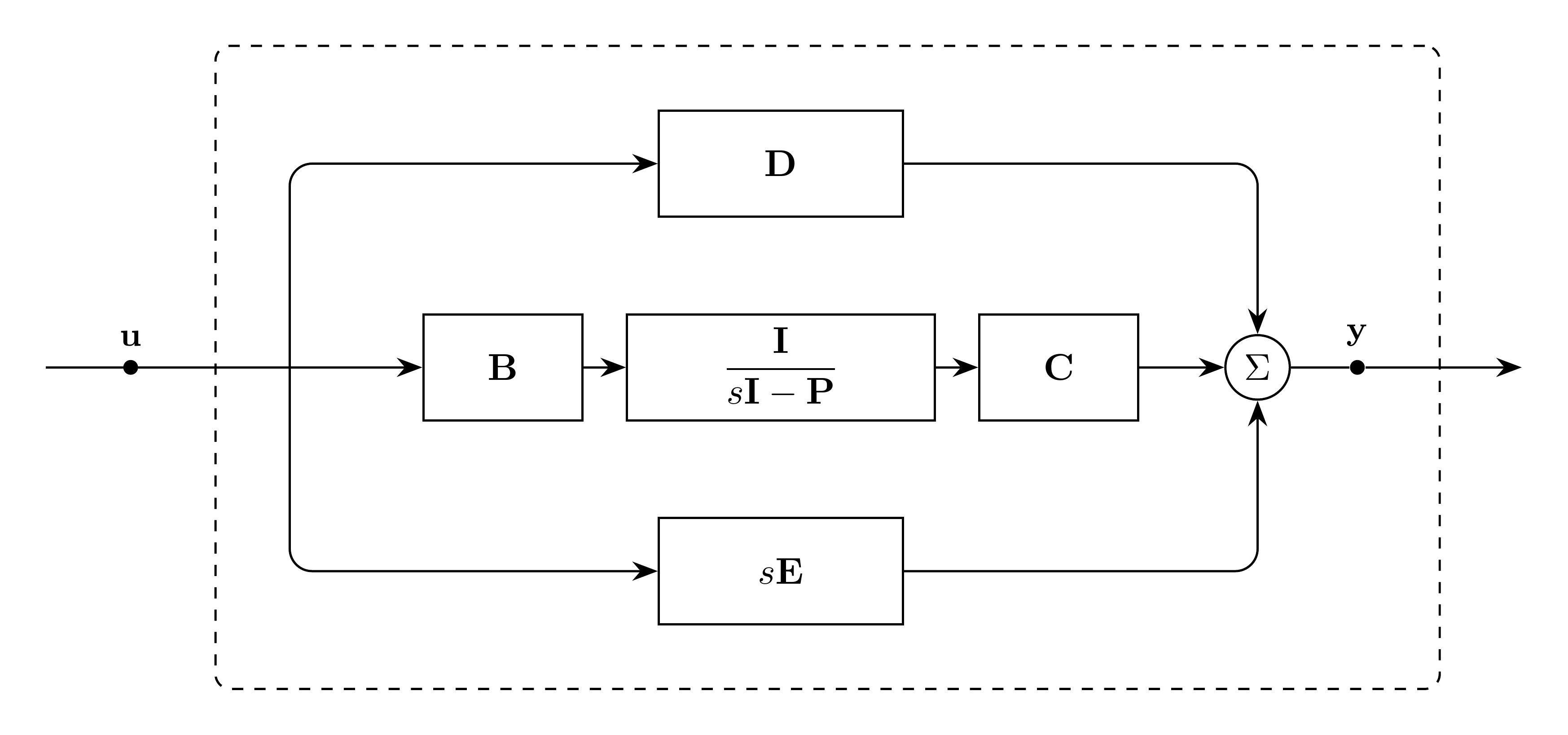
Figure 1: StateSpace model

Model Parameters

For output dimension \(N\), input dimension \(K\), pole count \(Q\), input units \([u]\), and output units \([y]\):

Symbol	Units	JSON	Description	Note
\(\mathbf{D}\)	\([y]/[u]\)	D	Constant coefficient	\(\mathbf{D} \in \mathbb{R}^{N \times K}\)
\(\mathbf{E}\)	\(\mathrm{s}[y]/[u]\)	E	Linear coefficient	\(\mathbf{E} \in \mathbb{R}^{N \times K}\)
\(\mathbf{p}\)	\([\mathrm{s}^{-1}]\)	poles	Poles	\(\mathbf{p} \in \mathbb{C}^Q\)
\(\mathbf{C}\)	\([y]/[u]\)	C	Output matrix	\(\mathbf{C} \in \mathbb{C}^{N \times Q}\)
\(\mathbf{B}\)	\([\mathrm{s}^{-1}]\)	B	Input matrix	\(\mathbf{B} \in \mathbb{C}^{Q \times K}\)

Parameter Validation

Let \(\mathcal{Q}_\mathrm{r} \subseteq \mathcal{Q}\) contain the real-pole indices and \(\mathcal{Q}_\mathrm{c} \subseteq \mathcal{Q}\) the first indices of the nonreal conjugate pairs. Define their partner-index set as

\[\mathcal{Q}_\mathrm{c}^{+} = \{q+1 \mid q \in \mathcal{Q}_\mathrm{c}\}\]

The sets \(\mathcal{Q}_\mathrm{r}\), \(\mathcal{Q}_\mathrm{c}\), and \(\mathcal{Q}_\mathrm{c}^{+}\) are pairwise disjoint.

\[\begin{split}\begin{aligned} N &\in \mathbb{Z}_{>0} \\ K &\in \mathbb{Z}_{>0} \\ Q &\in \mathbb{Z}_{\ge 0} \\ \mathbf{E} &= \mathbf{0}, \quad \text{for algebraic input} \\ \mathcal{Q}_\mathrm{r} \cup \mathcal{Q}_\mathrm{c} \cup \mathcal{Q}_\mathrm{c}^{+} &= \mathcal{Q} \\ p_q &\in \mathbb{R}, \quad \mathbf{C}_{:,q} \in \mathbb{R}^N, \quad \mathbf{B}_{q,:} \in \mathbb{R}^K, \quad q \in \mathcal{Q}_\mathrm{r} \\ p_{q+1} &= p_q^{\ast}, \quad q \in \mathcal{Q}_\mathrm{c} \\ \mathbf{C}_{:,q+1} &= \mathbf{C}_{:,q}^{\ast}, \quad q \in \mathcal{Q}_\mathrm{c} \\ \mathbf{B}_{q+1,:} &= \mathbf{B}_{q,:}^{\ast}, \quad q \in \mathcal{Q}_\mathrm{c} \end{aligned}\end{split}\]

Model Derived Parameters

\[\begin{split}\begin{aligned} \mathbf{P} &= \mathrm{diag}(p_1,\ldots,p_Q) \\ \mathbf{a} &= \mathrm{Re}(\mathbf{p}) \\ \boldsymbol{\omega} &= \mathrm{Im}(\mathbf{p}) \\ \mathbf{C}_r &= \mathrm{Re}(\mathbf{C}) \\ \mathbf{C}_i &= \mathrm{Im}(\mathbf{C}) \\ \mathbf{B}_r &= \mathrm{Re}(\mathbf{B}) \\ \mathbf{B}_i &= \mathrm{Im}(\mathbf{B}) \end{aligned}\end{split}\]

Model Ports

Symbol	Port	Type	Units	Description	Note
\(\mathbf{u}\)	input	Input	\([u]\)	Input vector port	\(\mathbf{u} \in \mathbb{R}^K\)
\(\mathbf{y}\)	out	Output	\([y]\)	Output vector port	\(\mathbf{y} \in \mathbb{R}^N\)

Submodels

None.

Submodel Validation

None.

Submodel Wiring

None.

Model Variables

Internal Variables

Differential

Symbol	Units	Description	Note
\(w_q\)	\([u]\)	Real memory state	\(w_q \in \mathbb{R}\), \(q \in \mathcal{Q}_\mathrm{r} \cup \mathcal{Q}_\mathrm{c}\)
\(v_q\)	\([u]\)	Imaginary memory state	\(v_q \in \mathbb{R}\), \(q \in \mathcal{Q}_\mathrm{c}\)

The documented real realization has order \(Q\).

Algebraic

None.

External Variables

Differential

Symbol	Units	Description	Note
\(\mathbf{u}\)	\([u]\)	Input vector	Differential-input configuration, \(\mathbf{u} \in \mathbb{R}^K\)

Algebraic

Symbol	Units	Description	Note
\(\mathbf{u}\)	\([u]\)	Input vector	Algebraic-input configuration, \(\mathbf{u} \in \mathbb{R}^K\)

Model Equations

Internal Equations

Differential

\[\begin{split}\begin{aligned} 0 &= -\dfrac{\mathrm{d}w_q}{\mathrm{d}t} + a_qw_q+\mathbf{B}_{q,:}\mathbf{u}, \quad q \in \mathcal{Q}_\mathrm{r} \\ 0 &= -\dfrac{\mathrm{d}w_q}{\mathrm{d}t} + a_qw_q-\omega_qv_q + (\mathbf{B}_r)_{q,:}\mathbf{u} \\ 0 &= -\dfrac{\mathrm{d}v_q}{\mathrm{d}t} + \omega_qw_q+a_qv_q + (\mathbf{B}_i)_{q,:}\mathbf{u}, \quad q \in \mathcal{Q}_\mathrm{c} \end{aligned}\end{split}\]

Algebraic

None.

External Equations

\[\mathbf{y} \leftarrow \mathbf{D}\mathbf{u} + \mathbf{E}\dfrac{\mathrm{d}\mathbf{u}}{\mathrm{d}t} + \sum_{q \in \mathcal{Q}_\mathrm{r}} \mathbf{C}_{:,q}w_q + 2\sum_{q \in \mathcal{Q}_\mathrm{c}} ((\mathbf{C}_r)_{:,q}w_q -(\mathbf{C}_i)_{:,q}v_q)\]

Initialization

None.

Monitors

None.