IEEET1

IEEE Type 1 excitation-system model.

Warning

Compensation impedance is not modeled.

Notes

• Voltage sensing uses the bus-voltage magnitude \(\sqrt{V_r^2 + V_i^2}\).

Block Diagram

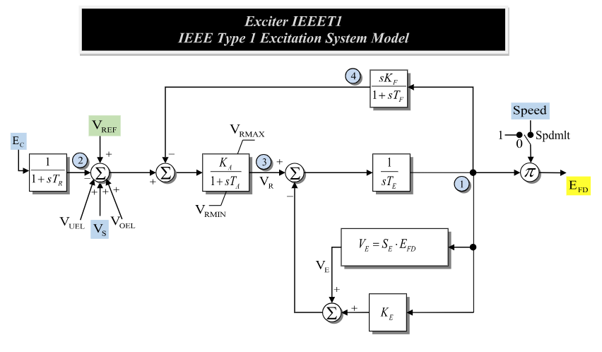
Figure 1: Exciter IEEET1 model. Figure courtesy of PowerWorld

Model Parameters

Symbol	Units	JSON	Description	Typical Value	Note
\(T_R\)	[s]	Tr	Time constant for voltage sensing	0
\(K_A\)	[p.u.]	Ka	Coefficient for voltage regulation	50
\(T_A\)	[s]	Ta	Time constant for voltage regulation	0.04
\(K_E\)	[p.u.]	Ke	Exciter field resistance line slope margin; 0 requests automatic calculation, not a zero coefficient	-0.06
\(T_E\)	[s]	Te	Time constant for excitation system	0.6
\(K_F\)	[p.u.]	Kf	Coefficient for feedback	0.09
\(T_F\)	[s]	Tf	Time constant for feedback	1.46
\(V_R^{\min}\)	[p.u.]	Vrmin	Lower limit to voltage regulation	-1
\(V_R^{\max}\)	[p.u.]	Vrmax	Upper limit to voltage regulation	1
\(E_1\)	[p.u.]	E1	Saturation Parameter	2.8
\(E_2\)	[p.u.]	E2	Saturation Parameter	3.73
\(S_1\)	[p.u.]	Se1	Saturation Parameter	0.04
\(S_2\)	[p.u.]	Se2	Saturation Parameter	0.33
\(I_{\mathrm{spdlim}}\)	[binary]	Ispdlim	Speed limit flag indicator	0

Parameter Validation

A valid IEEET1 parameter set must satisfy the following conditions:

\[\begin{split}\begin{aligned} \epsilon_T &= 10^{-3} \\ T &\leftarrow \max\!(T, \epsilon_T) \quad T \in \{T_R, T_A, T_E, T_F\} \\ K_A &> 0 \\ V_R^{\min} &\le V_R^{\max} \\ I_{\mathrm{spdlim}} &\in \{0,1\} \\ (S_1, S_2) &=(0,0) \quad\text{or}\quad \begin{gathered} E_1, E_2 > 0,\quad S_1, S_2 \ge 0 \\ (E_2-E_1)(S_2-S_1) > 0 \end{gathered} \end{aligned}\end{split}\]

Time constants below \(\epsilon_T\) are raised to \(\epsilon_T\) and logged as a warning; every other condition is a configuration error.

Model Derived Parameters

When saturation is disabled, \(S_A=0\) and \(S_B=0\). Otherwise, the parameters are chosen for the scaled-quadratic saturation model:

\[\begin{split}\begin{aligned} E S(E) &= S_B q(E-S_A) \\ E_1S_1 &= S_B(E_1-S_A)^2 \\ E_2S_2 &= S_B(E_2-S_A)^2 \\ \end{aligned}\end{split}\]

When exactly one saturation value is zero, the normal curve fit uses the corresponding voltage as the quadratic knee:

\[\begin{split}\begin{aligned} S_1=0 &: \quad S_A=E_1,\qquad S_B=\dfrac{E_2S_2}{(E_2-E_1)^2} \\ S_2=0 &: \quad S_A=E_2,\qquad S_B=\dfrac{E_1S_1}{(E_1-E_2)^2} \end{aligned}\end{split}\]

When both saturation values are positive, the non-extraneous solution is:

\[\begin{split}\begin{aligned} C &= \sqrt{ \dfrac {E_2S_2} {E_1S_1} } \\ S_A &= \dfrac {C E_1 - E_2} {C - 1} \\ S_B &= \dfrac {E_1S_1} {(E_1-S_A)^2} \end{aligned}\end{split}\]

\(K_E\) is the configured exciter field resistance line slope margin. A nonzero configured value is used directly. The IEEE Std 421.5-2016 states:

In some programs, if \(K_E\) is entered as zero, \(K_E\) is automatically calculated by the program to represent a self-excited shunt field and a trimmed rheostat as its initial condition.

GridKit implements the PSS/E-compatible automatic-parameter rule, as specified in the PSS/E 33.4 Program Application Guide, Vol. II. The divisor \(10\) in \(V_R=V_R^{\max}/10=0.1V_R^{\max}\) is unitless and sets \(V_R\) to 10% of the maximum regulator output, retaining the per-unit units of \(V_R^{\max}\):

\[\begin{split}\begin{aligned} 0 &= V_R -k_\mathrm{sat} -K_E^{\mathrm{eff}}E_{\mathrm{fd}}'\\ K_E^{\mathrm{eff}} &= \begin{cases} \dfrac{1}{E_{\mathrm{fd}}'} \left(\dfrac{V_R^{\max}}{10}-k_\mathrm{sat}\right) & K_E=0\\ K_E & K_E\ne 0 \end{cases} \end{aligned}\end{split}\]

Model Ports

Name	Port	Init	Description
bus	Bus	Known	Terminal bus voltage
speed	Input	Known	Machine speed deviation
vref	Input	Unknown	Voltage-control reference
vs	Input	Known	Stabilizer input signal
vuel	Input	Known	Under-excitation limiter input
voel	Input	Known	Over-excitation limiter input
efd	Output	Known	Field-voltage output seeded by the machine

Model Variables

Internal Variables

Differential

Symbol	Units	Description	Note
\(V_\mathrm{ts}\)	[p.u.]	Sensed terminal voltage
\(V_R\)	[p.u.]	Voltage regulator
\(E_{\mathrm{fd}}'\)	[p.u.]	Field voltage before the speed multiplier
\(V_\mathrm{fx}\)	[p.u.]	Exciter feedback internal state

Algebraic

Symbol	Units	Description	Note
\(V_{\mathrm{tr}}\)	[p.u.]	Terminal Voltage Error
\(V_\mathrm{f}\)	[p.u.]	Feedback Voltage
\(V_E\)	[p.u.]	Excitation control voltage
\(E_{\mathrm{fd}}\)	[p.u.]	Field winding voltage
\(k_\mathrm{sat}\)	[p.u.]	Scaled-quadratic saturation contribution	\(E_{\mathrm{fd}}'S(E_{\mathrm{fd}}')\)

External Variables

Differential

None.

Algebraic

Symbol	Units	Description	Note
\(V_r\)	[p.u.]	Real bus voltage component
\(V_i\)	[p.u.]	Imaginary bus voltage component
\(V_\mathrm{ref}\)	[p.u.]	Reference terminal voltage	Signal port vref
\(V_{\mathrm{uel}}\)	[p.u.]	Input from under excitation limiter	Signal port vuel
\(V_{\mathrm{oel}}\)	[p.u.]	Input from over excitation limiter	Signal port voel
\(V_S\)	[p.u.]	Input from stabilizer controller	Signal port vs
\(\omega\)	[p.u.]	Machine speed deviation	Signal port speed

Model Equations

Smooth functions: antiwindup, \(q\).

Internal Equations

Differential

For readability, define the pre-limit derivative of \(V_R\) and voltage-sensing input:

\[\begin{split}\begin{aligned} f_R &:= \dfrac{1}{T_A}(-V_R + K_A V_{\mathrm{tr}}) \\ E_C &:= \sqrt{V_r^2 + V_i^2} \end{aligned}\end{split}\]

The IEEET1 differential equations, as derived from the model diagram, are:

\[\begin{split}\begin{aligned} 0 &= -\dot V_\mathrm{ts} + \dfrac{1}{T_R}(E_C - V_\mathrm{ts}) \\ 0 &= -\dot V_R + \text{antiwindup} (V_R, f_R; V_R^{\min}, V_R^{\max}) \\ 0 &= -\dot E_{\mathrm{fd}}' + \dfrac{1}{T_E}(V_R - V_E - K_E^{\mathrm{eff}} E_{\mathrm{fd}}') \\ 0 &= -\dot V_\mathrm{fx} + \dfrac{1}{T_F}(V_\mathrm{f}) \end{aligned}\end{split}\]

Algebraic

\[\begin{split}\begin{aligned} 0 &= -V_\mathrm{ts} + V_\mathrm{ref} + V_{\mathrm{uel}} + V_{\mathrm{oel}} + V_S - V_{\mathrm{tr}} - V_\mathrm{f} \\ 0 &= -T_F(V_\mathrm{f} + V_\mathrm{fx}) + K_F E_{\mathrm{fd}}' \\ 0 &= -V_E + k_\mathrm{sat} \\ 0 &= -E_{\mathrm{fd}} + (1 + \omega I_{\mathrm{spdlim}})E_{\mathrm{fd}}' \\ 0 &= -k_\mathrm{sat} + S_B\, q(E_{\mathrm{fd}}' - S_A) \end{aligned}\end{split}\]

External Equations

None.

Initialization

The machine initializes \(E_{\mathrm{fd}}\) first. Set \(V_\mathrm{ref}\) to close the \(V_{\mathrm{tr}}\) equation:

\[\begin{split}\begin{aligned} E_C &\leftarrow \sqrt{V_r^2 + V_i^2} \\ E_{\mathrm{fd}}' &\leftarrow \dfrac{E_{\mathrm{fd}}}{1 + I_{\mathrm{spdlim}}\,\omega} \\ k_\mathrm{sat} &\leftarrow S_B\, q(E_{\mathrm{fd}}' - S_A) \\ V_E &\leftarrow k_\mathrm{sat} \\ V_R &\leftarrow K_E^{\mathrm{eff}} E_{\mathrm{fd}}' + V_E \\ V_{\mathrm{tr}} &\leftarrow \dfrac{V_R}{K_A} \\ V_\mathrm{fx} &\leftarrow \dfrac{K_F}{T_F}\, E_{\mathrm{fd}}' \\ V_\mathrm{ts} &\leftarrow E_C \\ V_\mathrm{f} &\leftarrow 0 \\ V_\mathrm{ref} &\leftarrow E_C + V_{\mathrm{tr}} - V_{\mathrm{uel}} - V_{\mathrm{oel}} - V_S \end{aligned}\end{split}\]

All internal derivatives initialize to zero.

Monitors

Monitor	Units	Description	Note
efd	[p.u.]	Field winding voltage
ksat	[p.u.]	Scaled-quadratic saturation contribution	\(S_B\,q(E_{\mathrm{fd}}'-S_A)\)